SKEDSOFT

Normal Distribution:

The perfectly smooth and symmetrical curve, resulting from the expansion of the binomial (q p) ⁿ when n approaches infinitely is known as the normal curve. Thus, the normal curve may be considered as the limit toward which the binomial distribution approaches as n increases to infinity. Alternatively we can say that the normal curve represents a continues and infinite binomial distribution when neither p nor q is very small. Even though p and q are not equal, for very large n we get perfectly smooth and symmetrical curve. Such curves are also called Normal Probability curve or Normal curve of Error or Normal Frequency curve. It was extensively developed and utilized by German Mathematician and Artsonomer Karl Gauss. This is why it called Gaussian curve in his honor. The normal distribution was first discovered by the English Mathematician Dr. A. De Moivre. Later on French Mathematician Pierre S. Laplace developed this principle. This principle was also used and developed by Quetlet, Galton and Fisher.

Assumptions of Normal Distribution:

The following are the four fundamental assumptions or conditions prevail among the factors affecting the individual events on which a normal distribution of observations is based:

1. Independent Factors: The forces affecting events must be independent of one another.

2. Numerous Factors: The causal forces must be numerous and of equal weight (importance).

3. Symmetry: The operation of the causal forces must be such that positive deviations from the mean are balanced as to magnitude and number by negative deviations from the mean.

4. Homogeneity: These forces must be the same over the population from which the observations are drawn (although their incidence will vary from event to event).

Equation of Normal Curve:

We obtain the theoretical frequencies for X = 0,1,2,3,.........n using the expansion N (q p)ⁿ. if p = q then binomial distribution becomes a symmetrical frequency distribution. When n is very large it is very difficult to compute the expected frequencies. This difficulty is overcome by normal curve. Normal curve is a continuous algebraic curve. Its formula is

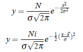
where y = computed height of an ordinate of the curve at a given point of x-series i,e. at a distance of x from the mean.

N = number of items in frequency distribution.

i = width of the class-interval.

σ = Standard deviation of the distribution.

Standard Normal Distribution:

It is useful to transform a normally distributed variable into such a form that a single table of areas under the normal curve would be applicable regardless of the unity of the original distribution. Let X be random variable distributed normally with mean ¯X and standard deviation σ , then we define a new random variable Z as;

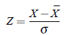
where Z = New random variable, X¯= value of X, X = Mean of X, σ = S.D. of X. Then Z is called a standard normal variate and its distribution is called standard normal distribution with mean 0 and standard deviation unity. Similarly we can obtain the values of Z for any given value of X as shown in the above figures.