SKEDSOFT
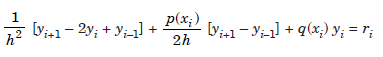
Using the approximations (1.3) and (1.4) in Eq.(1.58), we obtain
or,
 ................1.6
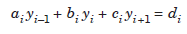
Collecting the coefficients, we can write the equation as
 ..................1.7
where,

Let us now apply the method at the nodal points. We have the following equations.
At x = x1, or i = 1:
 ..................1.8
At x = xi , i = 2, 3, …, n – 2 :
 .................1.9
At x = xn–1, or i = n – 1:
 ....................2.0
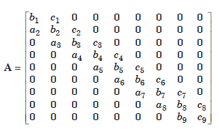
Eqs.(1.8), (1.9), (2.0) give rise to a system of (n – 1) × (n – 1) equations Ay = d for the unknowns y1, y2, ..., yi, ..., yn–1, where A is the coefficient matrix and

It is interesting to study the structure of the coefficient matrix A. Consider the case when the interval [a, b] is subdivided into n = 10 parts. Then, we have 9 unknowns, y1, y2, ....,y9, and the coefficient matrix A is as given.
Note :
It is a tri-diagonal system of algebraic equations. Therefore, the numerical solution of
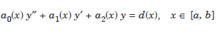
or,

by finite differences gives rise to a tri-diagonal system of algebraic equations, whose solution can be obtained by using the Gauss elimination method or the Thomas algorithm. Tri-diagonal system of algebraic equations is the easiest to solve. In fact, even if the system is very large, its solution can be obtained in a
few minutes on a modern desk top PC.