SKEDSOFT
The linear algebraic equations in a systematic manner, preferably in a way that can be easily coded for a machine. The best general choice is the Gauss-Jordan procedure which, with certain modifications that must be used to take into account problems arising from specific difficulties in numerical analysis, can be described very easily. Together with a couple of examples and a couple of exercises that you can do by following the given examples, it is easily mastered.
The idea is to start with a system of equations and, by carrying out certain operations on the system, reduce it to an equivalent system whose solution is easily found. It is based on three observations:
1. For a given system, it does not matter in which order the equations are listed;
2. The system remains unchanged if one equation is multiplied on both sides by a non-zero scalar;
3. If we alter replace one equation by the sum of that equation and a scalar multiple of another, then the system is unchanged.
These simple observations allow us to carry out a great simplification for any system of linear algebraic equations.
The method is based on the idea of reducing the given system of equations Ax = b, to a diagonal system of equations Ix = d, where I is the identity matrix, using elementary row operations. We know that the solutions of both the systems are identical. This reduced system gives the solution vector x. This reduction is equivalent to finding the solution as x = A-1b.
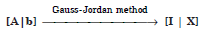
In this case, after the eliminations are completed, we obtain the augmented matrix for a 3 × 3 system as
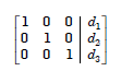 ....................1.1
and the solution is xi = di, i = 1, 2, 3.
Elimination procedure The first step is same as in Gauss elimination method, that is, we make the elements below the first pivot as zeros, using the elementary row transformations. From the second step onwards, we make the elements below and above the pivots as zeros using the elementary row transformations. Lastly, we divide each row by its pivot so that the final augmented matrix is of the form (1.42). Partial pivoting can also be used in the solution.
We may also make the pivots as 1 before performing the elimination.
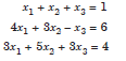
Example : Solve the following system of equations
using the Gauss-Jordan method (i) without partial pivoting, (ii) with partial pivoting
Solution We have the augmented matrix as

(i) We perform the following elementary row transformations and do the eliminations.
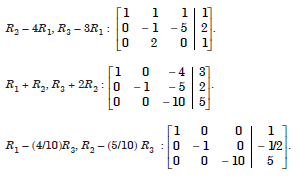
Now, making the pivots as 1, ((– R2), (R3/(– 10))) we get
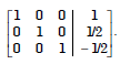
Therefore, the solution of the system is x1 = 1, x2 = 1/2, x3 = – 1/2.
