SKEDSOFT
Lagrange interpolation is a well known, classical technique for interpolation . It is also called Waring-Lagrange interpolation, since Waring actually published it 16 years before Lagrange . More generically, the term polynomial interpolation normally refers to Lagrange interpolation. In the first-order case, it reduces to linear interpolation.
Let the data
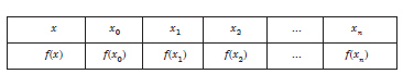
be given at distinct unevenly spaced points or non-uniform points x0, x1,..., xn. This data may also be given at evenly spaced points.
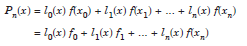
For this data, we can fit a unique polynomial of degree ≤ n. Since the interpolating polynomial must use all the ordinates f(x0), f(x1),... f(xn), it can be written as a linear combination of these ordinates. That is, we can write the polynomial as
 ....................1.1
where f(xi) = fi and li(x), i = 0, 1, 2, …,n are polynomials of degree n. This polynomial fits the data given in (1.1) exactly.
At x = x0, we get

This equation is satisfied only when l0(x0) = 1 and li(x0) = 0, i ≠ 0.
At a general point x = xi, we get

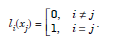
This equation is satisfied only when li(xi) = 1 and lj(xi) = 0, i ≠ j.
Therefore, li(x), which are polynomials of degree n, satisfy the conditions
 ....................1.2
Since, li(x) = 0 at x = x0, x1,..., xi-1, xi 1, ..., xn, we know that

are factors of li(x). The product of these factors is a polynomial of degree n. Therefore, we can write

where C is a constant.
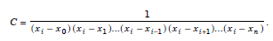
Now, since li(xi) = 1, we get

Hence,
Therefore,
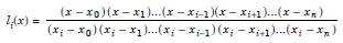 ....................1.3
Note that the denominator on the right hand side of li(x) is obtained by setting x = xi in the numerator.
