SKEDSOFT

CHALLENGES IN VALIDATING TIMING CONSTRAINTS IN PRIORITY-DRIVEN SYSTEMS
Compared with the clock-driven approach, the priority-driven scheduling approach has many advantages. As examples, you may have noticed that priority-driven schedulers are easy to implement. Many well-known priority-driven algorithms use very simple priority assignments, and for these algorithms, the run-time overhead due to maintaining a priority queue of ready jobs can be made very small. A clock-driven scheduler requires the information on the release times and execution times of the jobs a priori in order to decide when to schedule them. In contrast, a priority-driven scheduler does not require most of this information, making it much better suited for applications with varying time and resource requirements. You will see in later chapters other advantages of the priority-driven approach which are at least as compelling as these two.

Despite its merits, the priority-driven approach has not been widely used in hard realtime systems, especially safety-critical systems, until recently. The major reason is that the timing behavior of a priority-driven system is nondeterministic when job parameters vary. Consequently, it is difficult to validate that the deadlines of all jobs scheduled in a prioritydriven manner indeed meet their deadlines when the job parameters vary. In general, this validation problem [LiHa] can be stated as follows: Given a set of jobs, the set of resources available to the jobs, and the scheduling (and resource access-control) algorithm to allocate processors and resources to jobs, determine whether all the jobs meet their deadlines.

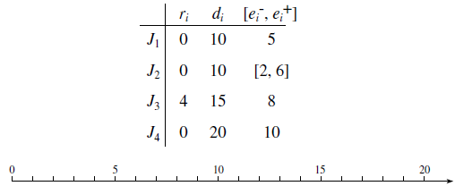
Anomalous Behavior of Priority-Driven Systems: Figure 4–8 gives an example illustrating why the validation problem is difficult when the scheduling algorithm is priority-driven and job parameters may vary. The simple system contains four independent jobs. The jobs are scheduled on two identical processors in a prioritydriven manner. The processors maintain a common priority queue, and the priority order is J1, J2, J3, and J4 with J1 having the highest priority. In other words, the system is dynamic. The jobs may be preempted but never migrated, meaning that once a job begins execution on a processor, it is constrained to execute on that processor until completion. (Many systems fit this simple model. For example, the processors may model two redundant data links connecting a source and destination pair, and the jobs are message transmissions over the links. The processors may also model two replicated database servers, and the jobs are queries dynamically dispatched by a communication processor to the database servers. The release times, deadlines, and execution times of the jobs are listed in the table.) The execution times of all the jobs are fixed and known, except for J2. Its execution time can be any value in the range [2, 6].

Suppose that we want to determine whether the system meets all the deadlines and whether the completion-time jitter of every job (i.e., the difference between the latest and the earliest completion times of the job) is no more than 4. A brute force way to do so is to simulate the system. Suppose that we schedule the jobs according their given priorities, assuming

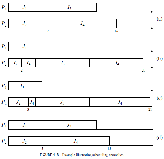
first that the execution time of J2 has the maximum value 6 and then that it has the minimum value 2. The resultant schedules are shown in Figure 4–8(a) and (b), respectively. Looking at these schedules, we might conclude that all jobs meet their deadlines, and the completiontime jitters are sufficiently small. This would be an incorrect conclusion, as demonstrated by the schedules in Figure 4–8(c) and (d). As far as J4 is concerned, the worst-case schedule is the one shown in Figure 4–8(c); it occurs when the execution time of J2 is 3. According to this schedule, the completion time of J4 is 21; the job misses its deadline. The best-case schedule for J4 is shown in Figure 4–8(d); it occurs when the execution time of J2 is 5. From this schedule, we see that J4 can complete as early as time 15; its completion-time jitter exceeds the upper limit of 4. To find the worst-case and best-case schedules, we must try all the possible values of e2.

The phenomenon illustrated by this example is known as a scheduling anomaly, an unexpected timing behavior of priority-driven systems. Graham [Grah] has shown that the completion time of a set of nonpreemptive jobs with identical release times can be later when more processors are used to execute them and when they have shorter execution times and fewer dependencies. (Problem 4.5 gives the well-known illustrative example.) Indeed, when jobs are nonpreemptable, scheduling anomalies can occur even when there is only one processor. For example, suppose that the execution time e1 of the job J1 in Figure 4–6 can be either 3 or 4. The figure shows that J3 misses its deadline when e1 is 3. However, J3 would complete at time 8 and meet its deadline if e1 were 4. We will see in later chapters that when jobs have arbitrary release times and share resources, scheduling anomalies can occur even when there is only one processor and the jobs are preemptable.

Scheduling anomalies make the problem of validating a priority-driven system difficult whenever job parameters may vary. Unfortunately, variations in execution times and release times are often unavoidable. If the maximum range of execution times of all n jobs in a system is X, the time required to find the latest and earliest completion times of all jobs is O(Xn) if we were to find these extrema by exhaustive simulation or testing. Clearly, such a strategy is impractical for all but the smallest systems of practical interest.

Predictability of Executions: When the timing constraints are specified in terms of deadlines of jobs, the validation problem is the same as that of finding the worst-case (the largest) completion time of every job. This problem is easy whenever the execution behavior of the set J is predictable, that is, whenever the system does not have scheduling anomalies. To define predictability more formally, we call the schedule of J produced by the given scheduling algorithm when the execution time of every job has its maximum value the maximal schedule of J. Similarly, the schedule of J produced by the given scheduling algorithm when the execution time of every job has its minimum value is the minimal schedule. When the execution time of every job has its actual value, the resultant schedule is the actual schedule of J. So, the schedules in Figure 4–8(a) and (b) are the maximal and minimal schedules, respectively, of the jobs in that system, and all the schedules shown in the figure are possible actual schedules.