SKEDSOFT
More Complex Control-Law Computations
The simplicity of a PID or similar digital controller follows from three assumptions. First, sensor data give accurate estimates of the state-variable values being monitored and controlled. This assumption is not valid when noise and disturbances inside or outside the plant prevent accurate observations of its state. Second, the sensor data give the state of the plant. In general, sensors monitor some observable attributes of the plant. The values of the state variables must be computed from the measured values (i.e., digitized sensor readings). Third, all the parameters representing the dynamics of the plant are known. This assumption is not valid for some plants. (An example is a flexible robot arm. Even the parameters of typical manipulators used in automated factories are not known accurately.)
When any of the simplifying assumptions is not valid, the simple feedback loop in Section 1.1.1 no longer suffices. Since these assumptions are often not valid, you often see digital controllers implemented as follows.
set timer to interrupt periodically with period T ;
at each clock interrupt, do
sample and digitize sensor readings to get measured values;
compute control output from measured and state-variable values;
convert control output to analog form;
estimate and update plant parameters;
compute and update state variables;
end do;
The last two steps in the loop can increase the processor time demand of the controller significantly. We now give two examples where the state update step is needed.
Deadbeat Control. A discrete-time control scheme that has no continuous-time equivalence is deadbeat control. In response to a step change in the reference input, a deadbeat controller brings the plant to the desired state by exerting on the plant a fixed number (say n) of control commands. A command is generated every T seconds. (T is still called a sampling period.) Hence, the plant reaches its desired state in nT second.
In principle, the control-law computation of a deadbeat controller is also simple. The output produced by the controller during the kth sampling period is given by
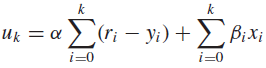
[This expression can also be written in an incremental form similar to Eq. (1.1).] Again, the constants α and βi ’s are chosen at design time. xi is the value of the state variable in the ith sampling period. During each sampling period, the controller must compute an estimate of xk from measured values yi for i ≤ k. In other words, the state update step in the above do loop is needed.
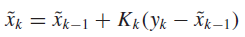
Kalman Filter. Kalman filtering is a commonly used means to improve the accuracy of measurements and to estimate model parameters in the presence of noise and uncertainty. To illustrate, we consider a simple monitor system that takes a measured value yk every sampling period k in order to estimate the value xk of a state variable. Suppose that starting from time 0, the value of this state variable is equal to a constant x. Because of noise, the measured value yk is equal to x εk , where εk is a random variable whose average value is 0 and standard deviation is σk . The Kalman filter starts with the initial estimate ˜ x1 = y1 and computes a new estimate each sampling period. Specifically, for k > 1, the filter computes the estimate ˜ xk as follows:
In this expression,
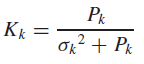
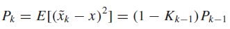
is called the Kalman gain and Pk is the variance of the estimation error ˜ xk − x; the latter is given by
This value of the Kalman gain gives the best compromise between the rate at which Pk decreases with k and the steady-state variance, that is, Pk for large k.
In a multivariate system, the state variable xk is an n-dimensional vector, where n is the number of variables whose values define the state of the plant. The measured value yk is an n' -dimensional vector, if during each sampling period, the readings of n' sensors are taken. We let A denote the measurement matrix; it is an n × n' matrix that relates the nxn measured variables to the n state variables. In other words,
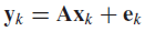
The vector ek gives the additive noise in each of the n' measured values. Eq. (1.2a) becomes an n-dimensional vector equation
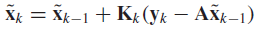
Similarly, Kalman gain Kk and variance Pk are given by the matrix version of Eqs. (1.2b) and (1.2c). So, the computation in each sampling period involves a few matrix multiplications and additions and one matrix inversion.
