SKEDSOFT
SIGNAL PROCESSING: Most signal processing applications have some kind of real-time requirements.We focus here on those whose response times must be under a few milliseconds to a few seconds. Examples are digital filtering, video and voice compressing/decompression, and radar signal processing.
Processing Bandwidth Demands: Typically, a real-time signal processing application computes in each sampling period one or more outputs. Each output x(k) is a weighted sum of n inputs y(i )’s:
In the simplest case, the weights, a(k, i )’s, are known and fixed.8 In essence, this computation transforms the given representation of an object (e.g., a voice, an image or a radar signal) in terms of the inputs, y(i )’s, into another representation in terms of the outputs, x(k)’s. Different sets of weights, a(k, i )’s, give different kinds of transforms. This expression tells us that the time required to produce an output is O(n).
The processor time demand of an application also depends on the number of outputs it is required to produce in each sampling period. At one extreme, a digital filtering application (e.g., a filter that suppresses noise and interferences in speech and audio) produces one output each sampling period. The sampling rates of such applications range from a few kHz to tens of kHz.9 n ranges from tens to hundreds. Hence, such an application performs 104 to 107 multiplications and additions per second.
Some other signal processing applications are more computationally intensive. The number of outputs may also be of order n, and the complexity of the computation is O(n2) in general. An example is image compression. Most image compression methods have a transform step. This step transforms the space representation of each image into a transform representation (e.g., a hologram). To illustrate the computational demand of a compression process, let us consider an m×m pixel, 30 frames per second video. Suppose that we were to compress each frame by first computing its transform. The number of inputs is n = m2. The transformation of each frame takes m4 multiplications and additions. If m is 100, the transformation of the video takes 3×10⁹ multiplications and additions per second! One way to reduce the computational demand at the expense of the compression ratio is to divide each image into smaller squares and perform the transform on each square. This indeed is what the video compression standard MPEG [ISO94]) does. Each image is divided into squares of 8 × 8 pixels. In this way, the number of multiplications and additions performed in the transform stage is reduced to 64m2 per frame (in the case of our example, to 1.92×10⁷). Today, there is a broad spectrum of Digital Signal Processors (DSPs) designed specifically for signal processing applications. Computationally intensive signal processing applications run on one or more DSPs. In this way, the compression process can keep pace with the rate at which video frames are captured.
Radar System
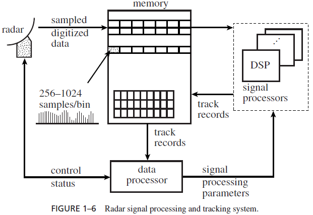
A signal processing application is typically a part of a larger system. As an example, Figure 1–6 shows a block diagram of a (passive) radar signal processing and tracking system. The system consists of an Input/Output (I/O) subsystem that samples and digitizes the echo signal from the radar and places the sampled values in a shared memory. An array of digital signal processors processes these sampled values. The data thus produced are analyzed by one or more data processors, which not only interface with the display system, but also generate commands to control the radar and select parameters to be used by signal processors in the next cycle of data collection and analysis.
Radar Signal Processing. To search for objects of interest in its coverage area, the radar scans the area by pointing its antenna in one direction at a time. During the time the antenna dwells in a direction, it first sends a short radio frequency pulse. It then collects and examines the echo signal returning to the antenna. The echo signal consists solely of background noise if the transmitted pulse does not hit any object. On the other hand, if there is a reflective object (e.g., an airplane or storm cloud) at a distance x meters from the antenna, the echo signal reflected by the object returns to the antenna at approximately 2x/c seconds after the transmitted pulse, where c = 3×10⁸ meters
per second is the speed of light. The echo signal collected at this time should be stronger than when there is no reflected signal. If the object is moving, the frequency of the reflected signal is no longer equal to that of the transmitted pulse. The amount of frequency shift (called Doppler shift) is proportional to the velocity of the object. Therefore, by examining the strength and frequency spectrum of the echo signal, the system can determine whether there are objects in the direction pointed at by the antenna and if there are objects, what their positions and velocities are.
Specifically, the system divides the time during which the antenna dwells to collect the echo signal into small disjoint intervals. Each time interval corresponds to a distance range, and the length of the interval is equal to the range resolution divided by c. (For example, if the distance resolution is 300 meters, then the range interval is one microsecond long.) The digital sampled values of the echo signal collected during each range interval are placed in a buffer, called a bin in Figure 1–6. The sampled values in each bin are the inputs used by a digital signal processor to produce outputs of the form given by Eq. (1.3). These outputs represent a discrete Fourier transform of the corresponding segment of the echo signal. Based on the characteristics of the transform, the signal processor decides whether there is an object in that distance range. If there is an object, it generates a track record containing the position and velocity of the object and places the record in the shared memory.
The time required for signal processing is dominated by the time required to produce the Fourier transforms, and this time is nearly deterministic. The time complexity of Fast Fourier Transform (FFT) is O(n log n), where n is the number of sampled values in each range bin. n is typically in the range from 128 to a few thousand. So, it takes roughly 103 to 105 multiplications and additions to generate a Fourier transform. Suppose that the antenna dwells in each direction for 100 milliseconds and the range of the radar is divided into 1000 range intervals. Then the signal processing system must do 107 to 109 multiplications and additions per second. This is well within the capability of today’s digital signal processors.
However, the 100-millisecond dwell time is a ballpark figure for mechanical radar antennas. This is orders of magnitude larger than that for phase array radars, such as those used in many military applications. A phase array radar can switch the direction of the radar beam electronically, within a millisecond, and may have multiple beams scanning the coverage area and tracking individual objects at the same time. Since the radar can collect data orders of magnitude faster than the rates stated above, the signal processing throughput demand is also considerably higher. This demand is pushing the envelope of digital signal processing technology.
